Predicting bank customer churn with ML
Classification models with Random Forest, AdaBoost and SVM
Customer churn prediction is a common application of data science and machine learning in business. It is useful for banks, telecommunications companies, SaaS products, marketing campaigns that turn leads into conversions and any business that relies on retaining customers as part of their model.
There are various nuances that can be added to improve the analysis but essentially it boils down to a classification problem, by predicting whether a customer would stop being one based on various features.
In this project, I analyse the transaction data of some customers in a bank, explore the distribution of various features, select the ones which have the most predictive value, train 3 classification models on the data and predict on a test set to compare the accuracies.
Data set
The dataset contains 10127 observations with 23 features – a mix of demographic, account, and transaction-related information such as:
- Attrition_Flag: A categorical variable indicating whether the customer has churned or not.
- Customer_Age, Gender, Dependent_count, Education_Level, Marital_Status, Income_Category and Card_Category
- Months_on_book: No. of months the customer has been on the books.
- Total_Relationship_Count: Total no. of products held by the customer.
- Credit_Limit: Credit limit of the customer.
- Total_Revolving_Bal: Total revolving balance on the credit card.
- Avg_Open_To_Buy: Average open to buy credit line (credit limit - total revolving balance).
- Total_Trans_Amt: Total transaction amount in the last 12 months.
- Total_Trans_Ct: Total transaction count in the last 12 months.
- Avg_Utilization_Ratio: Average utilization ratio of the credit card.
Data exploration
A quick exploration of the distribution of the features:
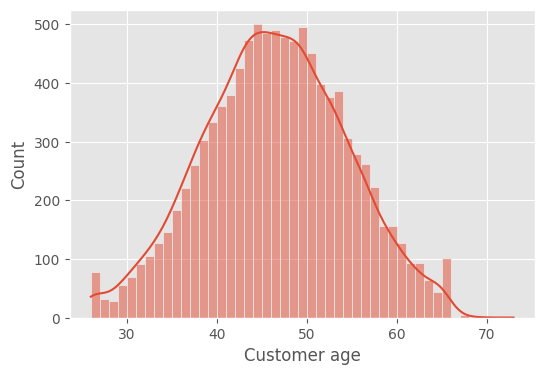
Age seems to be normally distributed.
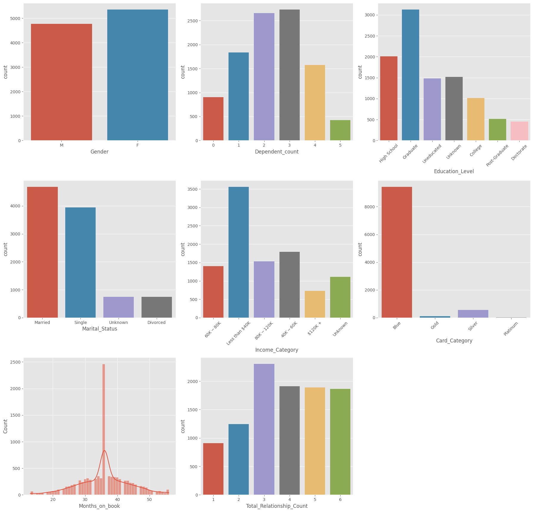
- There are more female customers in the sample than male. But the difference is not significant.
- Most common number of Dependents are 3, followed by 2 and then 1.
- Graduates make up the highest portion of customers, followed by those with a high school level of education. Education level of 15% of customers are unknown but even if they all have had no education, less than 30 (15+14.7) will fall under uneducated class. That means more than 70% of customers are educated at least until High School level.
- Almost half of the customers are married. And approximately the same Single (including Divorced).
- Highest proportion of customers have income less than 40K, followed by income in the range 40K to 60K.
- Blue card is the one with the most customers, followed by Silver.
- Months on book shows a peak of 36 months (3 years) with almost 25% (2500 out of 10127) customers being in the book for this period. There may have been a big campaign that attracted this cohort to become customers. The distribution does not seem to be normal.
- Fairly even distribution with 3 products being the most common, followed by 4. Since there is not much variation in this variable, it might not be a useful predictor of churn.
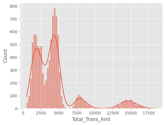
The distribution for Total_Trans_Amt (Total transaction amount in the last 12 months) seems to be multimodal. This suggests that there could be different distinct groups in the data, which could be helpful for a clustering task, to see what the differences between the groups are. It may have a direct influence on churn though.
Lastly, checking the distribution of the target variable reveals an imbalance.
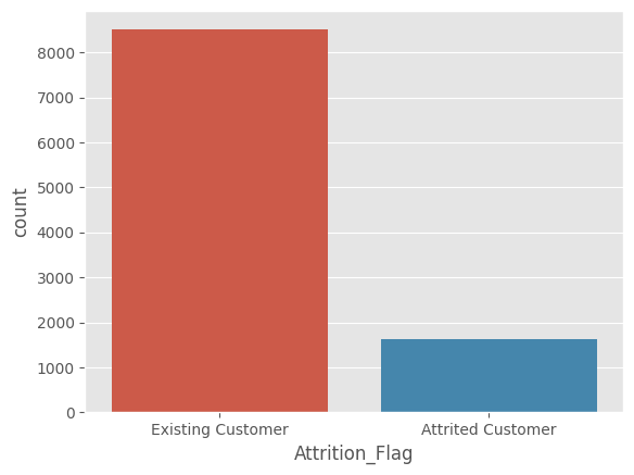
There are various techniques to deal with such imbalanced data, like oversampling (increasing number of examples from the minority class), undersampling (decreasing instances from majority class) and SMOTE (Synthetic Minority Over-sampling Technique), which involves generating synthetic samples for the minority class. In this case, I went with SMOTE since I wanted to keep as much of the available data as possible for training.
oversample = SMOTE()
X, y = oversample.fit_resample(data[data.columns[1:]], data[data.columns[0]])
upsampled = X.assign(Churn = y)
A few more steps before doing the training:
One-hot encode the categorical variables
The categorical variables are one-hot encoded using get_dummies, with one category of each dropped, along with the original categorical columns.
data = pd.concat([data,pd.get_dummies(data['Education_Level']).drop(columns=['Unknown'])],axis=1)
data = pd.concat([data,pd.get_dummies(data['Income_Category']).drop(columns=['Unknown'])],axis=1)
data = pd.concat([data,pd.get_dummies(data['Marital_Status']).drop(columns=['Unknown'])],axis=1)
data = pd.concat([data,pd.get_dummies(data['Card_Category']).drop(columns=['Platinum'])],axis=1)
data.drop(columns = ['Education_Level','Income_Category','Marital_Status','Card_Category'],inplace=True)
The target variable is also changed to a binary type.
data.Attrition_Flag = data.Attrition_Flag.replace({'Attrited Customer':1,'Existing Customer':0})
data.Gender = data.Gender.replace({'F':1,'M':0})
Checking for multicollinearity
If two features are highly correlated with each other, they provide redundant information. In this case, only one of them need to be used.
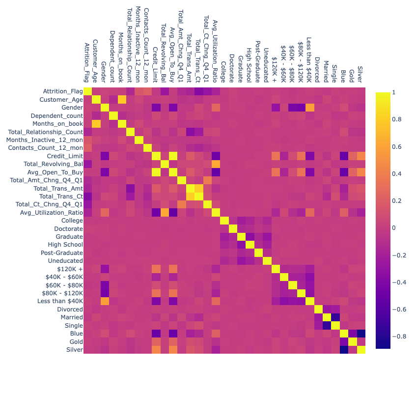
The only major correlations (above 0.5 in positive or negative direction) are
- Customer_Age and Months_on_book (0.79) : this makes sense as older customers likely have been with the bank longer
- Credit_limit and Avg_Open_To_Buy (1): Avg_Open_To_Buy is derived directly from Credit_limit (Credit_limit - balance), so they are perfectly correlated. Hence we can drop one of these.
- Total_Transaction_Amt and Total_Transaction_Ct (0.81): More transactions typically lead to higher total transaction amounts
- Total_Revolving_Bal and Avg_Utilization_Ratio (0.62): Higher revolving balances increase credit utilisation
- Gender and Less than $40K (0.58): Possibly one gender is more likely to earn less than 40K
Negatively correlated:
- Avg_Open_To_Buy and Avg_Utilization_Ratio (-0.54): Higher utilisation reduces available credit
- Credit_Limit and Blue (-0.52): “Blue” (e.g., a card type) might be associated with lower credit limits
- Avg_Open_To_Buy and Blue (-0.51): Similar to above, “Blue” may correlate with lower available credit
- Married and Single (-0.74): These are mostly mutually exclusive categories but maybe not perfectly correlated due to the other categories like Divorced
- Blue and Silver (-0.89): Likely mutually exclusive card types or tiers
Feature selection
And after the one-hot encoding, there were around 16 one-hot encoded categorical variables. To reduce the dimensionality, I used Principle Component Analysis (PCA) to bring these 16 down to 4.
Now there are a total of 19 features: 14 quantitative, 4 categorical and 1 target (Churn). The features which had the highest correlations with Churn, the target variable were:
Total_Trans_Ct              0.536860
PC-3                        0.451551
Total_Ct_Chng_Q4_Q1         0.393457
Total_Revolving_Bal         0.337962
Total_Relationship_Count    0.313742
Model training
After splitting the upsampled dataset into train and test with a 70-30 split, I created a pipeline which scales the features and trains the classifier models on the scaled features.
rf_pipe = Pipeline(steps =[ ('scale',StandardScaler()), ("RF",RandomForestClassifier(random_state=17)) ])
To compare the predictive capabilities of the model, I use f1 scores. F1 score is the harmonic mean of precision and recall, which means it balances both false positives and false negatives. This is also calculated with cross-validation using 5 folds, to reduce the variance associated with a single train-test split. The higher the F1 score, the better the prediction.
f1_cross_val_scores = cross_val_score(rf_pipe,X_train,y_train,cv=5,scoring='f1')
ada_f1_cross_val_scores=cross_val_score(ada_pipe,X_train,y_train,cv=5,scoring='f1')
svm_f1_cross_val_scores=cross_val_score(svm_pipe,X_train,y_train,cv=5,scoring='f1')
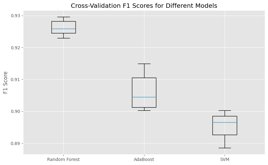
The Random Forest model produced the highest F1 scores. Using the trained models on the test dataset also yielded f1 scores in a similar order:
- Random Forest F1 Score: 0.93
- AdaBoost F1 Score: 0.90
- SVM F1 Score: 0.90
Just as a comparison, the predictions without oversampling were much lower in F1 scores:
- Random Forest F1 Score: 0.69
- AdaBoost F1 Score: 0.63
- SVM F1 Score: 0.62
Conclusion
This was a simple churn prediction task to predict which customers would churn based on various features that would be available as data collected by a bank. It involved exploration, one-hot encoding, checking for multi-collinearity, dimensionality reduction using PCA and feature scaling, followed by model training and evaluation on test set.
In real world projects, there could be be more complexity involved. For example, there could be instances of delayed churn, such as in the case of a cancellation that would go into effect at a much later date. This is where additional techniques like survival modelling can be useful.