Clustering binding sites based on distance and similarity metrics
ETL pipeline for exploring protein binding sites and similarity-based clustering
This was a continuation of my work with the research team under Dr. Petr Popov at Constructor University. In the first part of the project, I processed a collection of PDB files, computed the protein-ligand interaction fingerprints, explored their distributions including Gaussian smoothing and time series analysis followed by a visualization and an ETL pipeline to automate the whole workflow.
Following this, the research team was looking for ways to derive some patterns among various “binding sites” and “hotspots” in another collection of frames.
Binding sites are specific regions on a protein where small molecules - these could be drugs, ligands, or other biomolecules - can attach to interact with the protein. These sites influence the protein’s function, like how the protein behaves, how it interacts with other molecules, or how effective a drug can be. For e.g., in drug design, researchers often want to know exactly where a drug molecule binds on a protein to either block or activate a particular biological process.
Understanding these binding sites is central to structural bioinformatics. So in this project, I helped the research team find patterns among the various binding sites and hot spots. I proposed clustering the sites after representing them as numerical vectors, and based on comparable distance metrics, and finally creating a pipeline to automate the tasks from extraction to clustering and visualisations.
What I used
- Python in Visual Studio for extraction and analysis
- Standard data analysis packages - pandas, numpy
- scipy.stats, statsmodels, sklearn for statistical analysis and time series tests
- Packages & other tools for visualisation - matplotlib, seaborn, plotly
Data source and extraction
The data for this project came from precomputed .pkl files - one for each frame containing information about target structure and predicted binding sites with properties. Each .pkl file contained a dict with keys “target” and “sites”.:
- Binding site data, for example:
{'file': '0.pkl', 'site': { 'residues': ['A_14_GLY', 'A_15_VAL', ...], 'hotspots': [ {'center': array([44.39, 32.44, 13.74]), 'scores': {'small_molecule': 0.99}}, {'center': array([48.49, 33.62, 16.08]), 'scores': {'ion:-2': 0.59, 'ion:SO4': 0.46}} ] } } - Target data, for example:
{'file': '0.pkl',
 'target': {
  'chain_ids': [...],
  'atom_names': [...],
  'res_ids': [...],
  'coords': [...],
  'elements': [...]
 }}
Clustering methodology
In order to cluster the different binding sites, I first had to decide on the appropriate features. After discussing with the research team, I first had to represent each binding site by a “distance” metric. This could take one of three forms.
1. Residue overlap metric - a simple intersection of the sets of residues involved in two binding sites
def residue_overlap_distance(site1, site2):
    residues1 = set(site1.get('residues', []))
    residues2 = set(site2.get('residues', []))
    return 1 - len(residues1 & residues2) / len(residues1 | residues2)
2. Residue score metric - directly using the hotspot “scores” as feature vectors representing each binding site and finding the distance (Euclidean, L1, or Jaccard distance)
def residue_score_distance(site1, site2, distancetype):
    res_scores_1 = site1.get('residue_scores', {})
    res_scores_2 = site2.get('residue_scores', {})
    rnames = list(set.union(set(res_scores_1.keys()), set(res_scores_2.keys())))
    res_scores_1 = {**dict.fromkeys(rnames, 0), **res_scores_1}
    res_scores_2 = {**dict.fromkeys(rnames, 0), **res_scores_2}
    res_scores_1 = np.asarray(list(res_scores_1.values()), np.float32)
    res_scores_2 = np.asarray(list(res_scores_2.values()), np.float32)

    dist = np.sqrt(np.sum((res_scores_1 - res_scores_2) ** 2))

    return dist
3. Distance vector metric
This third approach is the most complex. It builds a consistent numerical representation of each binding site by encoding how its atoms relate to a global set of atoms of interest. This involved a few steps:
1. Identifying atoms in hotspots
A hotspot is essentially a functional region of a binding site. I needed to know exactly which atoms belonged to each hotspot. This involved mapping residue identifiers in a binding site to the corresponding atoms in the target structure. It ensures the right atoms are pulled out from the matching .pkl target file and records their details (chain ID, residue ID, atom name, element, and coordinates).
def get_atoms_in_binding_site(binding_site):
    file_name = binding_site['file']
    target= [entry for entry in all_target_data if entry['file'] in file_name] # extra check to make sure that the atoms are from the residues in the same pkl file
    target_data = next((entry for entry in target if entry['file'] == file_name), None)
    binding_site_residues = binding_site['site']['residues']
		parsed_residues = []
		for residue in binding_site_residues:
		        chain_id, res_id, res_name = residue.split('_')
		        parsed_residues.append((chain_id, int(res_id), res_name))

		chain_ids = target_data['target']['chain_ids']
		res_ids = target_data['target']['res_ids']
		res_names = target_data['target']['res_names']
		atom_names = target_data['target']['atom_names']
		coords = target_data['target']['coords']
		elements = target_data['target']['elements']

		atoms_in_site = []
		for chain_id, res_id, res_name in parsed_residues:
		    mask = (chain_ids == chain_id) & (res_ids == res_id) & (res_names == res_name)
		    matching_indices = np.where(mask)[0]

		    for idx in matching_indices:
		        atoms_in_site.append({
		            'chain_id': chain_id,
		            'res_id': res_id,
		            'res_name': res_name,
		            'atom_name': atom_names[idx],
		            'coords': coords[idx].tolist(),
		            'element': elements[idx],
		        })

		return atoms_in_site
2. Defining a global set of atoms
Once atoms are extracted from all binding sites, I collected them into a global catalogue of unique atoms by:
- Looping through all sites, runs, getting their atoms, and flattening the results
- Assigning each atom a unique identifier string, like “A_14_GLY_CA”
- Storing these unique atoms in an OrderedSet, which ensures that the feature vectors will always follow the same order
def atoms_of_interest(binding_sites):
    atoms_of_interest = []
    for site in binding_sites:
        atoms = get_atoms_in_binding_site(site)
        atoms_of_interest.append(atoms)
    all_atoms = [
        f"{atom['chain_id']}_{atom['res_id']}_{atom['res_name']}_{atom['atom_name']}"
        for atom_list in atoms_of_interest
        for atom in atom_list
        ]
    unique_atoms = OrderedSet(all_atoms) # Ordered set to maintain order in the calculation of the hotspot distances to atoms and binding vector for each site
    atoms_of_interest_flat = [atom for atoms in atoms_of_interest for atom in atoms]  # atoms_of_interest_flat has to be a dictionary
    print("Set of atoms of interest created (Distance Vector Method)")
    return unique_atoms, atoms_of_interest_flat
This global set of atoms was crucial: it defines the dimensions of the vector space in which all binding sites will be represented.
3. Looking up atom coordinates
I also wanted to retrieve the coordinates for any given atom ID. It searches through the global flat list of atom dictionaries (atoms_of_interest_flat) and returns the XYZ coordinates.
def get_atom_coordinates(atom_data):

    chain_id, res_id, res_name, atom_name = atom_data
    for entry in atoms_of_interest_flat:  # atoms_of_interest_flat has to be global and in a dictionary format
        if (
            entry['chain_id'] == chain_id and
            entry['res_id'] == int(res_id) and
            entry['res_name'] == res_name and
            entry['atom_name'] == atom_name
        ):
            return entry['coords']
    raise ValueError(f"Coordinates not found for atom: {atom_data}")
This step is what enables distance calculations later on.
4. Building the binding site vector
The heart of the method is binding_site_vector(binding_site, unique_atoms). For a given site, it constructs a fixed-length vector whose entries correspond to the global set of unique atoms.
Here’s the idea:
- Initialize the vector with a large dummy value (e.g. 10.0) for all atoms.
- For each hotspot in the binding site, compute the Euclidean distance between the hotspot center and the coordinates of each atom in the site.
- Update the vector entry for that atom with this distance.
Each hotspot generates its own vector. Then, for the final representation of the binding site, the code takes the minimum distance across all hotspots for each atom. This way, the binding site vector encodes the closest approach of its atoms to each hotspot.
def binding_site_vector(binding_site, unique_atoms):
    #dummy vector for all unique atoms with a large default value (e.g., 10.0) to keep vector lengths same, i.e. equal to length of unique atoms
    dummy_vector = {atom: 10.0 for atom in unique_atoms}
    residues_in_site = set(binding_site['site']['residues'])

    # get atoms from residues
    atoms_in_site = set(
        f"{atom['chain_id']}_{atom['res_id']}_{atom['res_name']}_{atom['atom_name']}"
        for atom in atoms_of_interest_flat
        if f"{atom['chain_id']}_{atom['res_id']}_{atom['res_name']}" in residues_in_site
    )

    hotspot_vectors = []
    for hotspot in binding_site['site']['hotspots']:
        hotspot_coords = hotspot['center']
        hotspot_vector = dummy_vector.copy()

        for atom in unique_atoms.intersection(atoms_in_site):
            atom_data = atom.split('_')
            atom_coords = get_atom_coordinates(atom_data)
            distance = np.linalg.norm(np.array(hotspot_coords) - np.array(atom_coords))
            hotspot_vector[atom] = distance # updates the distance for only that element of the hotspot vector where the id matches this particular atom

        # add the hotspot vector to the list of vectors
        hotspot_vectors.append(hotspot_vector)

    # Calculate the binding site vector as the minimum distance across all hotspots for each atom
    binding_site_vector = [
        min(hotspot_vector[atom] for hotspot_vector in hotspot_vectors) for atom in unique_atoms
    ]

    return binding_site_vector
The result is a dense numerical vector of equal length for all binding sites, ready for pairwise comparison
Computing the distance between 2 distance vectors and distance matrix
Once I had site vectors, it was just a matter of computing the distance (using (L2/Euclidean or L1/Manhattan etc.) between 2 vectors to get this third type of distance metric.
For each type of distance metric, it was necessary to compute a distance matrix. The distance matrix is a 2D array where entry (i, j) represents the distance between binding site i and binding site j. And although the binding sites themselves are the “items” being clustered, each row in the distance matrix corresponds to a binding site, and the algorithm assigns a cluster label to that row.
def pairwise_distances_with_library(sites, distance_func, distance_type):
    def distance_wrapper(i, j, distance_type):
        return distance_func(sites[int(i[0])], sites[int(j[0])], distance_type)

    indices = list(range(len(sites)))
    condensed_matrix = pdist([[i] for i in indices], metric=lambda i, j: distance_wrapper(i, j, distance_type))

    return squareform(condensed_matrix)

def calculate_distance_matrix(binding_sites, distance_metric, distance_type):
        if distance_metric == 'residue_overlap':
            return pairwise_distances_with_library(binding_sites, residue_overlap_distance, distance_type)
        elif distance_metric == 'residue_score':
            return pairwise_distances_with_library(binding_sites, residue_score_distance, distance_type)
        elif distance_metric == 'distance_vector':
            global unique_atoms, atoms_of_interest_flat
            unique_atoms, atoms_of_interest_flat = atoms_of_interest(binding_sites)
            return pairwise_distances_with_library(binding_sites, distance_between_vectors, distance_type)

distance_matrix = calculate_distance_matrix(binding_sites, distance_metric, distance_type)
This is unlike traditional clustering applications in “business” where a product or item is assigned a cluster based on its features. In fact, you can think of the distance matrix as a collection of items with their features, except the items themselves are entire rows (binding sites) and the features are the columns. Or in other words, instead of using the raw attributes of a binding site, we use its pattern of distances to every other binding site as its effective “feature vector.”
Clustering Algorithms
For each distance metric, I used four clustering algorithms as the research team wanted the flexibility of using anyone of them based on their needs.
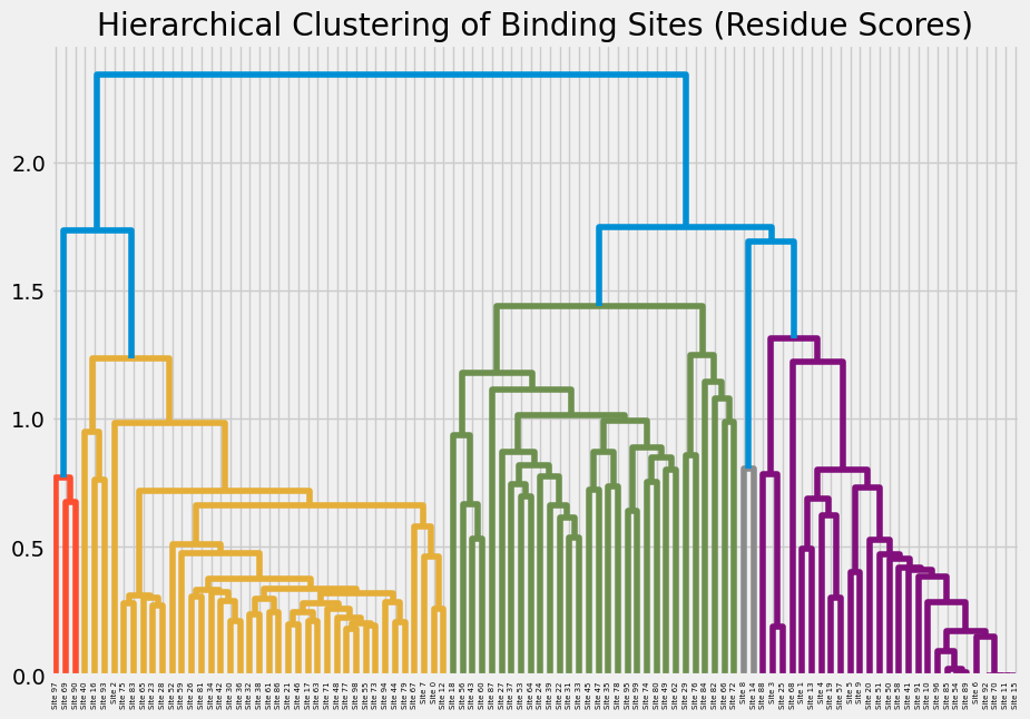
Agglomerative Clustering
Builds a hierarchy of clusters by repeatedly merging the closest pair of sites. Best for small to medium datasets where the hierarchy itself is meaningful.
agglom_model = AgglomerativeClustering(n_clusters=len(clusters), metric='precomputed', linkage=linkage_method)
cluster_labels = agglom_model.fit_predict(distance_matrix)

DBSCAN
Groups sites that are close together in dense regions and labels isolated points as noise. This is good when you suspect that some binding sites don’t really belong to any cluster but shouldn’t be forced into one.
dbscan = DBSCAN(metric='precomputed', eps=epsilon, min_samples=minimum_samples)
dbscan_labels = dbscan.fit_predict(distance_matrix)
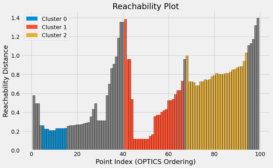
OPTICS
Similar to DBSCAN, but more flexible. Instead of fixing one density threshold, this explores clusters across a range of densities and produces a reachability plot.
 optics = OPTICS(metric='precomputed', min_samples=5, xi=xi, min_cluster_size=minimum_cluster_size)
optics_labels = optics.fit_predict(distance_matrix)

MeanShift
Shifts points toward the densest regions in the data until stable clusters form. It doesn’t need you to predefine the number of clusters, and it’s a good choice when clusters are expected to be roughly “blob-shaped” around centres.
mean_shift = MeanShift()
mean_shift_labels = mean_shift.fit_predict(distance_matrix)
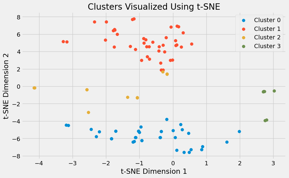
Since binding site vectors are high-dimensional, t-SNE plots can help project them down into 2D for visualization.
For example:
embedding = TSNE(n_components=2, metric='precomputed', init='random').fit_transform(distance_matrix)
        plt.figure(figsize=(10, 6))
        for cluster_id in np.unique(cluster_labels):
            cluster_points = embedding[cluster_labels == cluster_id]
            plt.scatter(cluster_points[:, 0], cluster_points[:, 1], label=f'Cluster {cluster_id}', s=50)
        plt.title('Clusters (Agglomerative) visualized Using t-SNE')
        plt.xlabel('t-SNE Dimension 1')
        plt.ylabel('t-SNE Dimension 2')
        plt.legend()
        plt.show()
Points that end up close together in the plot are generally similar in the original feature space, giving an intuitive view of cluster separation.

Deploying into production with an ETL pipeline
Once the logic and workflow was agreed on, the research team wanted a configurable pipeline where they could:
- Choose the metric type (residue_overlap, residue_score, or distance_vector) and for each of these, additional parameters like options normalisation: min, max, average, or union.
- Select the distance metric (Euclidean, Manhattan, cosine, Jaccard, etc.)
- Experiment with different clustering algorithms (hierarchical, KMeans, DBSCAN, HDBSCAN)
- Control other parameters like the subset of binding sites, dimensionality reduction method, or output visualisations
To support this, I built a single production-ready Python file (clustering_pipeline.py) that functions as an ETL pipeline:
- Extraction - with functions for loading binding site and atom data from the provided .pkl files. And also for handling mapping atoms and constructing the unique atom identifiers.
- Transformation - functions to calculate the
- residue_overlap_distance, residue_score_distance and distance_between_vectors for the 3 methods, each taking in 2 sites as arguments. The 3rd function also depended on other helper functions like:
- get_atoms_in_binding_site, atoms_of_interest (to list all unique atoms from all binding sites in all files), get_atom_coordinates (to get coordinates for atom specified)and binding_site_vector (to calculate the vector for a binding site based on the distances between hotspots and unique atoms)
- pairwise_distances_with_library – builds pairwise distance matrices between binding sites for the chosen distance metric.
- Loading & Analysis
- perform_clustering (that takes in the distance_matrix and other clustering_args ) – applies the chosen clustering algorithm (hierarchical, KMeans, DBSCAN, HDBSCAN) and generates t-SNE plots for visualization, while also returning the clustering labels
- a mapping function that takes in the binding site (or a subset of the binding site for testing calculations quickly) and clustering labels to output a JSON file that pairs the binding site with the cluster label.
def mapping(subset, labels):
    labels = [int(label) for label in labels]
    subset_with_labels = [
        {"residues": site["site"].get("residues", []), "cluster_label": label}
        for site, label in zip(subset, labels)
    ]
    output_file = "bindingsites_with_labels.json"
    with open(output_file, "w") as f:
        json.dump(subset_with_labels, f, indent=4))
So the output JSON would contain elements like this:
[
    {
        "residues": ["A_14_GLY", "A_15_VAL", ...],
        "cluster_label": 0
    },
    {
        "residues": ["A_20_SER", "A_21_THR", ...],
        "cluster_label": 1
    },
    ...
]
- Configuration Layer
- A core function “cluster” to take in a JSON file path as the argument, which contains all the parameters for the pipeline such as the location of the folder with the pkl files, a subset to analyse if needed, distance metric types, and specifically what type of distance (Euclidean, Manhattan, Jaccard etc.), clustering algorithm, number of clusters, and other clustering parameters). The clustering parameters JSON file could look something like this:
{
"path_to_pkl_files": "/path/to/pkl-folder/kras_md_sites_1",
"subset_to_analyse": 50,
"distance_metric": {
  "metric_type": "distance_vector",
  "distance_type": "jaccard"
},
"clustering_model": {
  "type": "optics",
  "parameters": {
"min_samples": 5,
 "xi": 0.05,
 "min_cluster_size": 0.1
  }
}
}
- A core function “cluster” to take in a JSON file path as the argument, which contains all the parameters for the pipeline such as the location of the folder with the pkl files, a subset to analyse if needed, distance metric types, and specifically what type of distance (Euclidean, Manhattan, Jaccard etc.), clustering algorithm, number of clusters, and other clustering parameters). The clustering parameters JSON file could look something like this:
- Main Function
- The *main* function which orchestrates the end-to-end pipeline, accepting the path to the JSON file as input and calling the cluster function with this JSON file path to run the entire workflow.
if __name__ == '__main__':
  parser = argparse.ArgumentParser(description="Cluster binding sites from PKL files (frames)")
  parser.add_argument('--json_path', type=Path, help="Path to the folder containing the JSON files with the parameters")
  args = parser.parse_args()
  print(f"Folder Path: {args.json_path}")
  cluster(args.json_path)
This structure allowed the research team to test out with different settings and parameters without editing the codebase — they only need to update the JSON configuration file.
- The *main* function which orchestrates the end-to-end pipeline, accepting the path to the JSON file as input and calling the cluster function with this JSON file path to run the entire workflow.
Some challenges and lessons from this project
- The data extraction: The JSON files accompanying the PDB data included multiple layers of nested dictionaries and lists, containing various residues, targets and their properties and metrics
- The subject matter: Initially, it was hard to wrap my head around the goal of the task, and what binding sites and targets were. The complex JSON structures in the data files did not make things easier. I had to discuss with the research team and subject matter experts in detail a few times before getting clarity.
- Representation matters: A binding site isn’t naturally a vector - deciding whether to use residue overlap, hotspot scores, or atom distances fundamentally changes the clustering.
- Cluster count variability: MeanShift might found 3 clusters while Agglomerative found 19 - not “wrong”, just a reflection of different assumptions.
- Mapping back to binding sites: After clustering, the key was mapping each binding site back to its residues/atoms to interpret what the clusters actually represent.
- The ETL pipeline: This was tricky due to the number of helper functions involved and how they depended on each other. But testing with smaller subsets for quick checks got me there eventually.