Time series forecasting for non-transparent markets (wood waste)

Time series forecasting methods are commonly used in transparent markets stocks and other financial instruments where prices are openly disclosed and relevant information about market conditions, product specifications and other factors influencing transactions are readily accessible.

There are other markets though, such as wood waste, where information is not as easily available, and where there are various other external factors which make prediction of future values challenging.

In this project, I helped a market-leading firm in Germany forecast future prices using a variety of time series forecasting models. The firm supplies combined heat and power plants with the desired combustibles including waste wood. Their business model relies on collecting wood waste from sellers, which could be consumers or businesses, at a specific price and selling it to power plants for energy generation. This makes it critical for the company to know what the price of the wood waste will be in the future, in order to understand and arrive at an appropriate number for negotiations.

Tech used

• Python in Visual Studio
• Time series analysis and related necessary packages

Data collection and preprocessing

The data used for this analysis and forecasting was provided by the client. It includes the price of waste as recorded by them weekly from around Sep 2020 until May 2024. The price value is sometimes recorded as negative, which is when the client was paid for taking the waste from the supplier and at other times as positive, in which case the client made payments to suppliers to take the waste from them.

There were 5773 observations in total in the data set, with seven columns for distinct features. These include among others:

• A “week” column in object type
• “wPreis” which contains the price recorded in float format
• “Plz” which is a string object that denotes the cluster (combination of Postal Codes)
• “Category” – a string object that denotes one category of the wood waste
• “Behandelt” – a string object that denotes another category of the wood waste
• “full” – a string object that denotes the combination of the Category and Behandelt categories

The data is recorded for 10 unique clusters which are collections of Postal Codes (Postleitzahl) in Germany, like [‘25’, ‘24’], [‘80’, ‘81’, ‘82’, ‘83’, ‘84’, ‘85’, ‘93’, ‘94’], [‘70’, ‘71’, ‘73’, ‘74’, ‘75’, ‘76’] and so on.

The category variables are just different categories of the wood waste as recorded by the client. There were no null values in the data set so it was not required to drop any rows.

Some basic cleaning steps included some string edits and transformations to simplify the category column and conversion of the ‘week’ column to datetime format.

The “full” category is simply the combination of the values in the Category and Behandelt columns, which makes the latter two columns redundant and these could be removed.

Since the week variable contained only week numbers in the format “YYYY-WW” denoting the number of the week in the year, this is converted into a datetime variable in the format “YYYY-MM-DD”. As a general best practice for time series analysis and prediction, the datetime variable is also set as the index of the dataframe.

Data exploration

When the wPreis values were plotted, it was seen that for all 3 categories in the same cluster these values followed a somewhat similar trend, with occasional deviations. The number of categories in each cluster also varied, as some clusters have only one waste category, such as ‘A1 & A2 -  geschreddert’ for the cluster [1, 4, 6, 7, 8, 9] while others can have up to 6 categories like the cluster  [‘40’, ‘41’, ‘42’, ‘44’, ‘45’, ‘46’, ‘47’].

There could be a number of factors behind this structure for these time series. If one had to hypothesize, one could say that the gradual increase in 2020 could be in part due to the post-COVID-19 recovery and resumption of economic activities, which may also have had an effect on the demand for wood-based products. The sharp rise in early to mid 2020 may have been driven by the energy crisis, exacerbated by geopolitical tensions, and the increased demand for alternative energy sources, including biomass and wood waste, not to mention the rising inflation rates. The subsequent drops in prices from the middle of 2022 may have resulted in part due to the stabilisation of supply chains as producers and suppliers adjusted to the increased demand, as well as the economic slowdown or recession in 2023.

**Time series modelling **

For this project, I used the following time series models for forecasting.

• ARIMA
• Decision Trees
• Random Forest
• XGBoost
• Prophet

Wherever possible in each of these models, I also explored different procedures of forecasting – namely Static (multi-step), Rolling window, and Walk-forward validation.

• Static (Multi-step) Forecasting: This involves fitting the model on a training subset of historical data and generating forecasts for multiple future time steps corresponding to a test subset in one go. The model is trained using a fixed historical window once, and forecasts are generated for a predefined horizon.
• Rolling Window Forecasting: In this method, the model is fit to the training data set in a rolling window of pairs of X and y values. The forecast is made one step at a time based on the input from the immediately preceding window taken as predictors. The window rolls forward incorporating new observations from the test data set to predict for the next step, while discarding older data points. (Note that this procedure of forecasting was not applicable for all the models under consideration due to various reasons, including the fact that some models do not take a sequence as input or in the case of Prophet, the design of the model as publicly released by Facebook)
• Walk-forward Validation: Here, the model is trained with an increasing historical window and used to generate forecasts for the next single time step. The forecasting for each step in the test data set is still done based on a moving window of preceding input but the historical window is not fixed but continues to grow larger.

Auto-correlation and Partial Auto-correlation

Before testing the different models on the time series, especially that of autoregressive models like ARIMA, it is important to consider whether there are any correlations in the structure of the data. The Auto-correlation Function (ACF) and Partial Auto-correlation Function (PACF) allow us to choose appropriate lags and inputs that models need to be supplied with as parameters for prediction.

The ACF measures how correlated the values of a time series are with those at a different time in the series, known as lagged values. The PACF is a similar metric, which also examines the correlation between values in a time series and its lags while also taking into account the effects of the time steps in between.

The plotting functions plot_acf, plot_pacf from the statsmodels.graphics.tsaplots package can be used to plot both the ACF and the PACF. When these plotting functions are called on the price values for the categories in the cluster [‘25’, ‘24’] the following results can be observed.

The ACF plots show that there is a positive correlation with the first 10-to-15 lags and it decreases backwards in time until it becomes less significant after around 15 weeks. The PACF plots show high correlation for 1 week lag but that is expected. There are also significant correlations for lags up to and around 5, as well as further back in time, around 20 weeks.

Seasonal decomposition

In addition to the ACF and PACF, it is also useful to decompose the time series into three main components – Trend, Seasonality and Residuals – a process called seasonal decomposition

Similar to the ACF and PACF, the functions seasonal_decompose from the from statsmodels.tsa.seasonal can be used to extract the trend, seasonal and residual components. For the “period” parameter, I chose 4, based on what the ACF and PCF plots suggested to be lags worth considering.

When applied on the price values for the cluster [‘25’, ‘24’] and for the category ‘A1 & A2 - geschreddert’ we observe the following components.

The seasonality also shows that there is a clear seasonal pattern around 4 weeks, although the scale of the seasonal changes are small compared to that of the trend

Stationarity – Testing and Converting

Another important step that must be taken before time series modeling, especially in the case of the ARIMA model, is the check for stationarity. A stationary time series is one in which the statistical properties such as mean and variance stay constant over time.

Checking for stationarity is crucial for determining the appropriate modelling approach as some models such as ARIMA assume stationarity. To check for stationarity there are statistical tests such as the Augmented Dickey-Fuller (ADF) test.

Differencing

Converting a time series to stationary can be achieved with differencing. This involves computing the differences between consecutive observations. The result is a stabilization of the mean of the time series by removing changes in the level, and therefore reducing trend and seasonality.

The ADF test is performed by using the adfuller function from the statsmodels.tsa.stattools package. Performing the ADF test again on this 1st differenced time series gives the following results.

Since the test statistic in this case is much less than all the critical values, it means that the null hypothesis has been rejected and that this time series is stationary.

Applying the test for all the categories and clusters showed that most were non-stationary and had to be differenced. While the 1st order differencing was seen to convert the time series of some of the categories to stationary, for some categories such as A2 & A3 - geschreddert in [‘50’, ‘51’, ‘52’, ‘53’], A2 & A3 - ungeschreddert in [‘40’, ‘41’, ‘42’, ‘44’, ‘45’, ‘46’, ‘47’] and A3 - geschreddert in [‘40’, ‘41’, ‘42’, ‘44’, ‘45’, ‘46’, ‘47’] are not stationary even after 1st differencing. However, one second order differencing, they are all detected as stationary.

Hence, wherever applicable in the modelling (such as ARIMA models), the difference order of 2 can be taken.

Modeling

To account for the possible difference in the number of observations across all the time series (across clusters and categories), the training test split is based on a ratio of 95-5 % ratio.

The main parameters I used for evaluation were:

• rmse: Root Mean Squared Error, the square root of the square of the difference between between the actual values in the test set and that predicted by the model.
• Direction accuracy: Quantifies the fraction of the number of times that the model predictions were in the right direction (up or down) as the change in the expected values.

ARIMA

The ARIMA model combines three key components: Autoregression (AR), Integration (I), and Moving Average (MA).

Autoregression refers to how the current value depends on past values. Integration represents the differencing operation applied to the time series data to make it stationary. The Moving Average (MA) component of ARIMA captures the dependency between the current value of the series and the residual errors from previous predictions. It models the short-term fluctuations in the data.

The model is generally denoted by ARIMA(𝑝,𝑑,𝑞) where the parameters are lag (p), differencing (d) and residual error (q).

Choice of p and d for ARIMA

As seen from the ADF tests and differencing steps, the value of d can be taken as 2. To arrive at a single value of p for standardizing the predictions and comparing across all categories and clusters, the AIC values for p values up to 10 are compared as below.

Getting the predictions for the cluster [‘25’, ‘24’] and for the category ‘A1 & A2 - geschreddert’ using static and walk-forward validation method gives the following:

Static

Walk-forward

Decision Tree

Decision trees are non-parametric supervised learning methods which work by partitioning the feature space into a set of disjoint regions based on recursive binary splitting of the feature space. At each step, the algorithm selects the feature and the split point that optimally separates the data according to some criterion, such as maximizing information gain or minimizing impurity. For time series forecasting, decision trees can be adapted by incorporating lagged variables as features. When this is done in each of the forecasting methods for the cluster [‘25’, ‘24’] and for the category ‘A1 & A2 - geschreddert’ I got the following results.

Static

Rolling

Walk-forward

Random Forest

Random Forest is an ensemble learning technique that combines the predictions of multiple decision trees to improve overall performance. It works by constructing a collection of decision trees, each trained on a random subset of the training data and a random subset of the input features. It is based on the bootstrap aggregation (bagging, which involves the creation of decision trees, where each is constructed from a different bootstrap sample in the training dataset. A bootstrap sample is one where an observation may appear more than once in the sample. This means that decision tree is fit on a slightly different training dataset, which gives slightly different performance for each. Predictions from the trees are averaged across all decision trees, to produce better performance than that given by any single tree.

When this is done for the cluster [‘25’, ‘24’] and for the category ‘A1 & A2 - geschreddert’ within it gives the following results.

Static

Rolling

Walk-forward

XGBoost

XGBoost, which stands for eXtreme Gradient Boosting, is an efficient implementation of gradient boosting that builds a collection of decision trees sequentially, with each subsequent tree focusing on correcting the errors made by the previous ones in an iterative approach. By employing gradient boosting techniques, XGBoost optimizes the learning process by iteratively adding new trees that minimize a specified loss function.

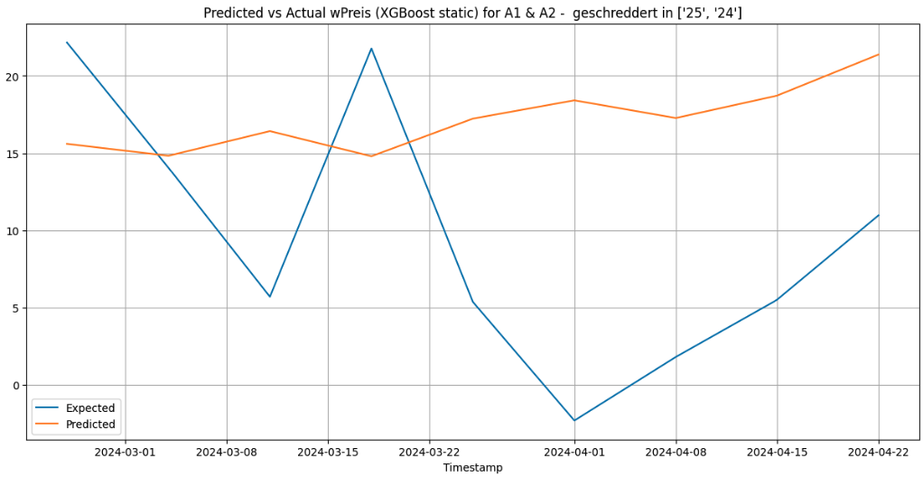
When XGBoost is used with the 3 forecasting methods for the cluster [‘25’, ‘24’] and for the category ‘A1 & A2 - geschreddert’, it gives the following results:

Static

Rolling

Walk-forward

Prophet

Prophet is a time series forecasting model developed by Facebook that is based on an open-source library. It is designed to automatically find a good set of hyperparameters in order to make accurate forecasts for data with trends and seasonal structure. It is known to be able to fit with yearly, weekly, and daily seasonality, plus holiday effects and therefore is capable of forecasting data with strong seasonal patterns, multiple seasonality, and holidays.

Using Prophet, the 3 forecasting methods for the same cluster and category yielded the following results:

Static

Walk-forward

Insights

The results of forecasting using each of the available methods for ARIMA, Decision Tree, Random Forest, XGBoost and Prophet models illustrate the following points.

• Static forecasting methods usually perform worse than others

For the specific category of A1 & A2 - geschreddert for the cluster [‘25’, ‘24’], the Prophet model with the walk-forward validation forecasting has the lowest RMSE among all (7.94) followed closely by the XGBoost model with the rolling window forecasting (7.97) and the XGBoost model with the walk-forward validation method (8.23).

In all models, the static forecasting approach had higher RMSE, suggesting that either a rolling window or walk-forward validation method is likely to be preferable in general if the objective is to forecast values of wPreis as closely as possible to the real values that will be observed.

Direction accuracy, which can often be a more useful metric for stakeholders interested in planning ahead for price increases or decreases, is the highest for Decision Tree model when forecasting is done with the walk-forward validation (62%) and all others are accurate at most 50% of the time.

• Different time series may require different methods and models

As seen from the evaluation of the different methods for each of the models ARIMA, Decision Trees, RandomForest, XGBoost and Prophet and the various methods of forecasting using each, there is no clear winner that applies for all the categories and clusters. The complete comparison of RMSE values for each of the model-method combination for each of the time series(which can be viewed in the Appendix) shows this clearly. In fact, counting the number of times each model-method combination produced the lowest RMSE in all of the 33 time series, the following counts can be obtained.

As seen from the above plot, the walk-forward validation method using ARIMA model produced the lowest RMSEs most times (7) out of all the 33 time series, followed by the rolling forecast method using Decision Tree (5) and the walk-forward method using Prophet (4) times. Similarly, in the case of the highest direction accuracy among all model-method combination, the static forecasting using Decision Tree was the best in 7 out of the 33 time series, followed by the static forecasting using ARIMA (6) and Random Forest (5). Thus there is no single best model or indeed, the specific forecasting method within each model that can be applied universally across all time series and different categories and clusters may require specific choices of models and methods for the best predictive capabilities.